Machine Learning Week 2 - Octave Tutorial - グラフ描画
Machine Learning Week 2 - Octave Tutorial - 基本操作 の続き
グラフ描画は色々詰まる要素が多かった。。。
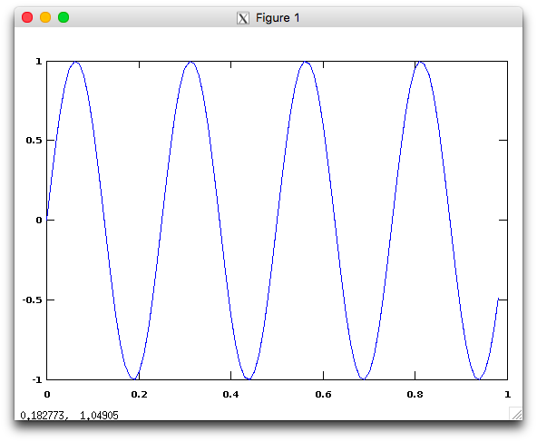
簡単なグラフ描画
データを準備すればplotコマンドでグラフ描画できる.
❯❯ t = [0:0.01:0.98];
❯❯ y1 = sin(2*pi*4*t);
❯❯ plot(t,y1);
エラー等でうまく表示してくれない場合は、.octavercの設定ができてない可能性がある。Machine Learning - Octaveの導入を参考に.octavercを作成のこと
複数のグラフ描画
別々のウィンドウで表示
figureコマンドを使用する事で名前付けできる
❯❯ figure(1); plot(t,y1);
❯❯ figure(2); plot(t,y2);
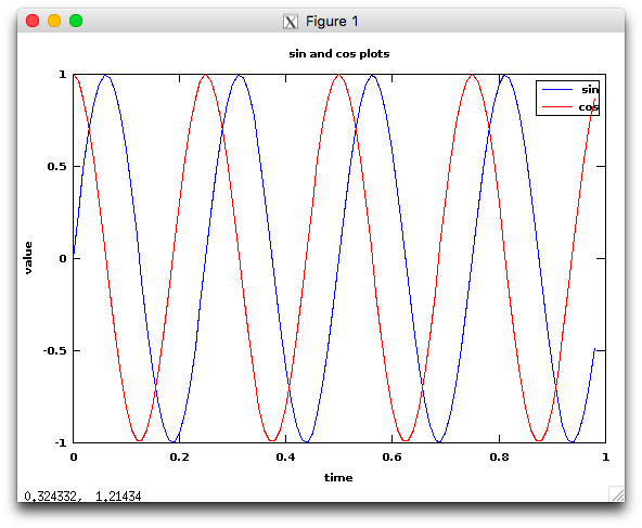
グラフを一つのウィンドウに描写
hold onコマンドを使えば、以降に表示するグラフが元の図に追加されていく
❯❯ y2 = cos(2*pi*4*t);
❯❯ plot(t,y1);
# hold onコマンドで、これ以降のグラフも同一グラフに表示できる
❯❯ hold on;
# 2つ目のグラフ描写
❯❯ plot(t,y2,'r');
# x方向のラベル名を指定
❯❯ xlabel('time')
# y方向のラベル名を指定
❯❯ ylabel('value')
# 各線の説明を追加
❯❯ legend('sin', 'cos')
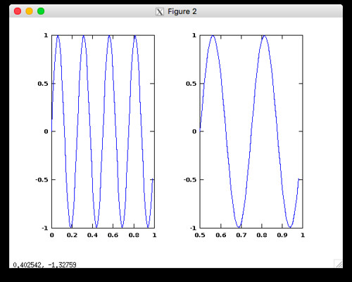
グラフを一つにウィンドウに描写(分割)
subplotを使えば、一つの画面に複数のグラフを同時に描写できる
❯❯ subplot(1,2,1)
❯❯ plot(t,y1);
❯❯ subplot(1,2,2)
❯❯ plot(t,y1);
❯❯ axis([0.5 1 -1 1])
グラフの画像出力
printコマンドでグラフ描画できるが、最初以下のようなエラーメッセージがでて出力できなかった.
❯❯ print -dpng 'myplot.png'
warning: print.m: fig2dev binary is not available.
Some output formats are not available.
warning: called from
    __print_parse_opts__ at line 385 column 9
    print at line 288 column 8
❯❯
原因はpng出力時に利用しているfig2devが足りなかったからで、homebrewでインストールする場合は以下でできる.
 $ brew install homebrew/x11/imake
 $ brew tap mistydemeo/homebrew-xfig
 $ brew install transfig
しかしこれでprintしたら、出力グラフが真っ黒になってしまった。
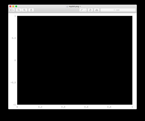
原因はgnuplot5にある模様. 2015/11/19時点ではバグは治ってないようなので、png出力したい場合はgnuplotを4にしておく必要あり.
It seems there is a problem with gnuplot 5 and Macs (see the bug report). I was able to solve this by doing as suggested in the link and downgrading to gunplot version 4.6.6
octave on OSX Yosemite, print outputs doc, but graph is solid black - Stack Overflow
gnuplotのバージョンダウン
グラフをpng出力したい場合は、以下のコマンドでgnuplotを5.0.1から4.6.6にする
$ brew uninstall gnuplot
$ brew install homebrew/versions/gnuplot4 --with-aquaterm --with-x11
eps方式で出力したい場合
更にpngではなくeps形式で出力したい場合は、brewの設定ファイルを弄ってインストールが必要な模様。けど現時点でeps形式で出す必要はないので今回は無視。
ここで開いたファイルの「inreplace」が連続しているところの末尾に
inreplace "fig2dev/dev/genibmgl.c", "static set_width(w)", "static void set_width(w)"
を追加してください。
グラフクリア
❯❯ clf
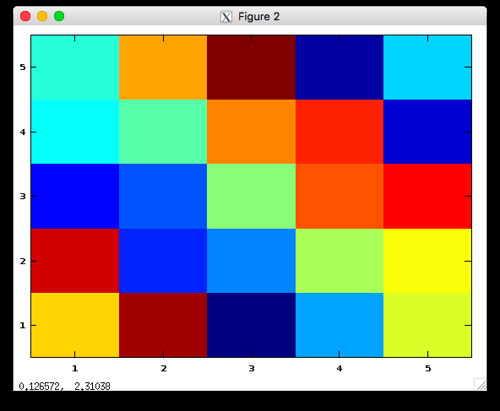
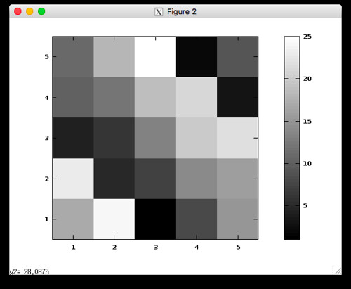
グリッドカラー表示
これはちょっとおもしろかった
❯❯ A = magic(5);
❯❯ imagesc(A)
# カラーバー+グレースケール表示
❯❯ imagesc(A), colorbar, colormap gray;
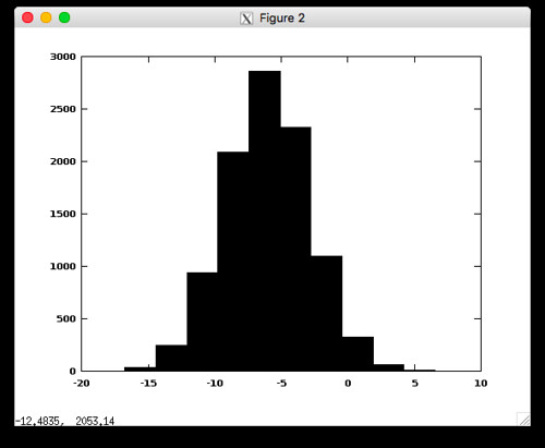
ヒストグラム
histでヒストグラムも一瞬.
# randnは単純なランダムではなく、正規分布に基づくランダム値が主力される
❯❯ w = -6 + sqrt(10)*(randn(1,10000));
❯❯ hist(w)